Neuron Identification and Segmentation

This research was sponsored and supported by the Wu Tsai Institute (WTI).

Working with the Liang Lab at Yale University, our computational neuroscience lab analyzed the neural firing patterns in the visual system both in temporal and spatial domains using Convolutional Neural Networks (CNNs).

This approach aimed to help researchers simplify the manual detection and segmentation of firing neurons. This research was built on work done by Bao et al. 2021. Mapping brain activity to stimulus involves stimulating neurons relevant to the visual system in mice in-vivo through optogenetic techniques. By counting neurons, we can understand whether the correct neural pathways were activated.

Neuron Identification in the Visual Thalamus:

• Identifying and segmenting neurons in video spatially and temporally yields important insights about the visual system.
• Manual identification and segmentation of neurons is difficult and time-consuming, especially for multi-frame images.
• Deep neural networks have reached a point of achieving human-level (or better) accuracy in this task.

The lab also was interested in the creation of a computational framework to iteratively improve upon our machine learning model.

Main Goals

1. Revamp calcium imaging workflow pipeline
   • Update and optimize the existing calcium imaging workflow to enhance the detection and analysis of neuron activity.
   • Incorporate advanced techniques to accurately capture in-vivo neuron firing patterns, improving the resolution and reliability of the data.
     
     
2. Deployment of CNN-based machine learning neuron segmentation framework
   • Implement a Convolutional Neural Network (CNN) framework to automate the segmentation of neurons in calcium imaging data.
   • Enhance the accuracy and efficiency of identifying active neurons during in-vivo stimulation, ensuring precise mapping of neural pathways.
     
     
3. Run tests on different imaging conditions
   • Conduct comprehensive testing of the updated workflow and CNN framework under various imaging conditions.
   • Evaluate performance across different light intensities, imaging depths, and stimulation protocols to ensure robustness and adaptability in capturing in-vivo neuron firing.
     

Convolutional Neural Networks

CNNs are pivotal in the field of artificial intelligence, particularly for tasks involving image and video recognition, medical image analysis (useful for us), and natural language processing. Their importance lies in their ability to automatically and adaptively learn spatial hierarchies of features from input images, making them highly effective for identifying patterns and objects in visual data. Unlike traditional neural networks, CNNs leverage convolutional layers to preserve the spatial relationships within the data, enabling more accurate and efficient processing. There are many iterations of CNNs–and as will be seen in our work–a specific iteration of CNNs known as UNets will be utilized.

This unique capability makes CNNs indispensable for applications ranging from autonomous driving, where real-time object detection is crucial, to healthcare, where they assist in diagnosing diseases from medical imaging. Their robustness, scalability, and high accuracy in pattern recognition underscore the transformative impact CNNs have on technology and various industries.

Figure 1 below shows how CNNs can be used for classifications tasks. On the left, we see a mall hallway with people walking around. The goal in this toy example is to identify and count how many people are in the hallway at any given time. On the right, we see how an inference step through this example CNN model can identify locations of people by representing them with a red dot. We will expand on this functionality to meet our needs in a bit.

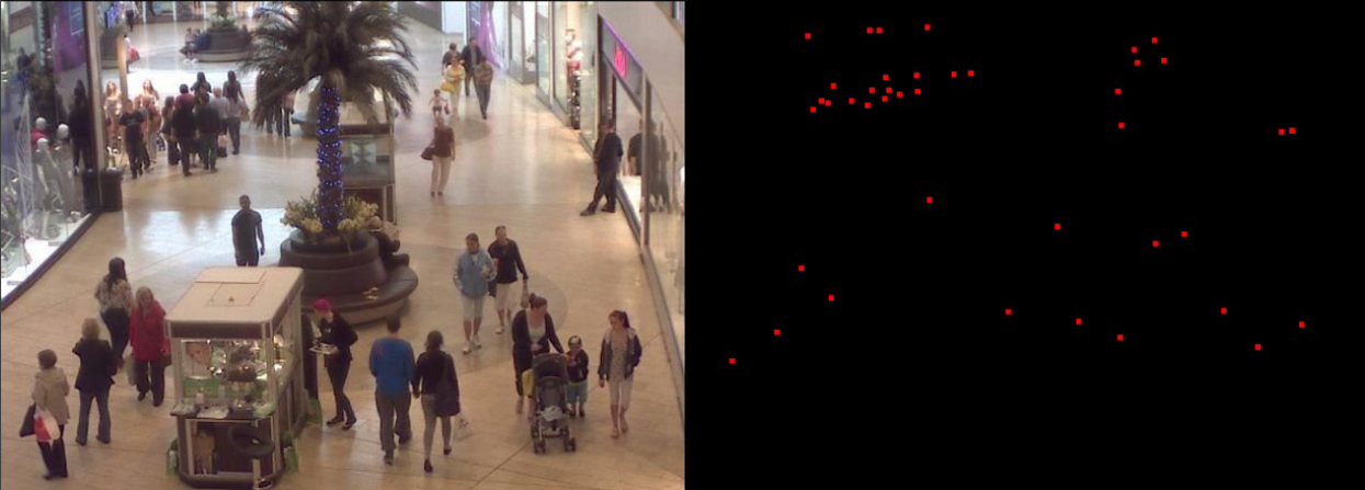
Figure 2 below illustrates the critical features of a Convolutional Neural Network (CNN) and its process for image recognition. Initially, the network takes an input image, in this case, a car. As the image passes through the network, it undergoes a series of convolutional layers designed to extract different levels of features. The first layers capture low-level features such as edges and textures, represented by simple patterns like lines and gradients. These low-level features are combined and processed through deeper layers to form more complex, high-level features, such as parts of objects like wheels, headlights, and car bodies. Finally, these high-level features are fed into fully connected layers that integrate the extracted information and produce a final output, here identifying the car as a “Volvo XC90.” This hierarchical approach enables CNNs to effectively learn and recognize intricate patterns within images, making them exceptionally powerful for various computer vision tasks. This classification ability builds on the toy example of crowd detection and counting above (Figure 1).

Additionally, Figure 3 shows how filters are applied within each stage (or layer) of the CNN shown in Figure 2. This depends on multiple factors as the equation shown in Figure 4. This article gives good insight into this mathematical process.

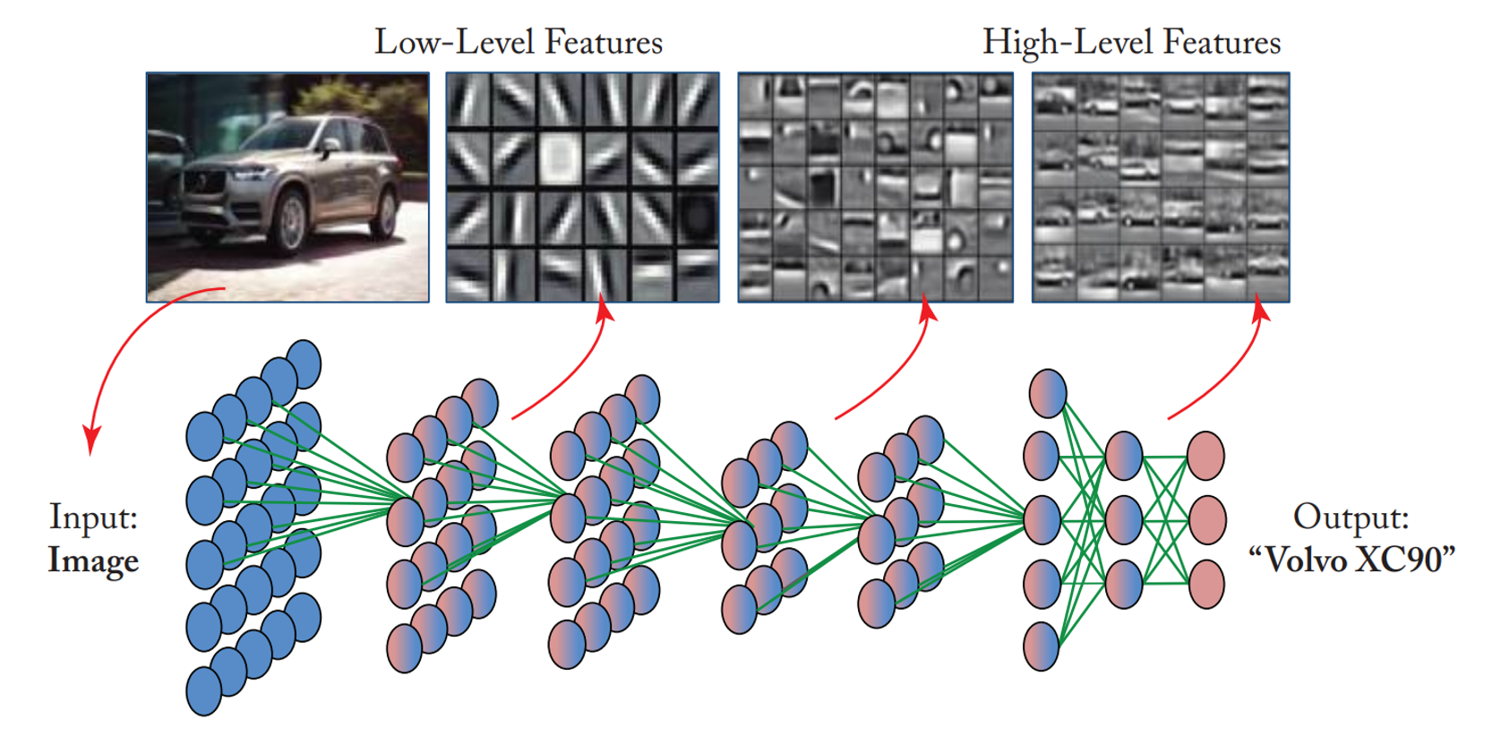
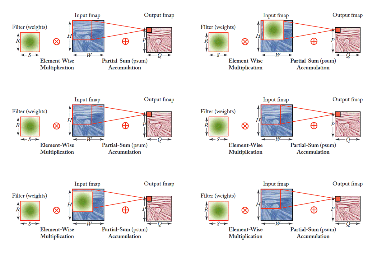
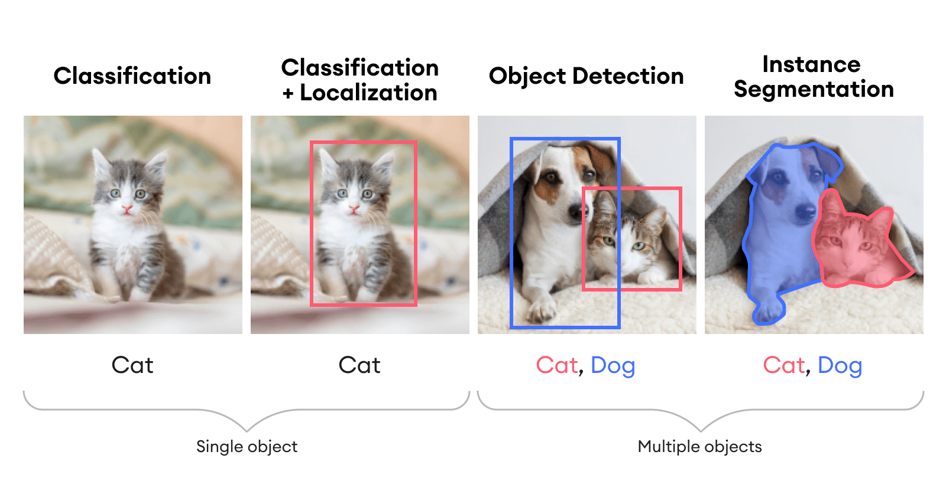
Figure 5 demonstrates the different tasks within computer vision, highlighting the capabilities of advanced neural network models in understanding and interpreting visual data:

• Classification
  • Identifies and labels the main object in an image.
  • Example: Recognizes a single object such as a “Cat.”
• Classification + Localization
  • Identifies and labels the main object in an image and provides the object’s location using a bounding box.
  • Example: Recognizes a “Cat” and draws a bounding box around it.
• Object Detection
  • Identifies, labels, and provides the locations of multiple objects within an image using bounding boxes.
  • Example: Recognizes both a “Cat” and a “Dog” and draws bounding boxes around each.
• Instance Segmentation
  • Identifies, labels, and precisely delineates the boundaries of multiple objects within an image.
  • Example: Recognizes both a “Cat” and a “Dog” and highlights their exact shapes with colored masks.

Each task progresses in complexity, from merely recognizing what is in the image to accurately locating and segmenting multiple objects within the image. This will be the theoretical basis for our neuron detection and segmentation task. Of course, this becomes complicated when attempting to detect and segment thousands of firing neurons through many iterative frames; these examples will be unable to capture these complexities. Thankfully, our lab was able to find a unique UNet architecture, a superset of base CNN architectures. We will expand on this soon.

UNet CNN Architecture

The importance of U-Net architecture in medical imaging lies in its exceptional ability to segment images accurately, even with limited data. U-Net excels in tasks requiring precise localization and delineation of structures within medical images. Its ability to accurately reconstruct high-resolution images from compressed representations makes it ideal for medical applications, where detail and accuracy are critical for diagnosis and treatment planning.

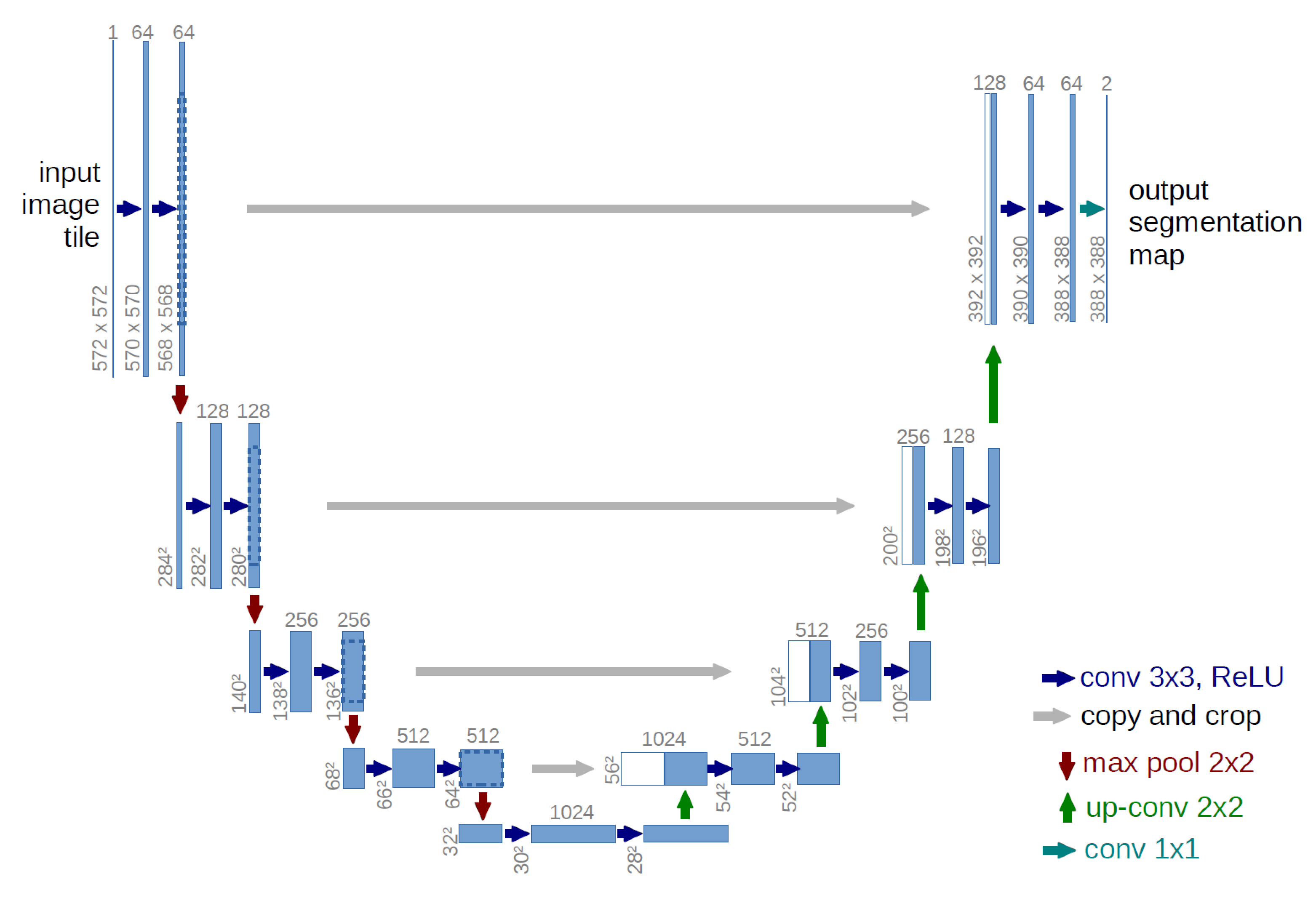
As such, in order to eachive these goals, the U-Net architecture employs the encoder/decoder framework. The encoder part is a network (commonly found as fully-connected, CNN, RNN, etc). In our case, it is a CNN due to our requirement for imaging inference capability. Both the encoder and decoder work hand-in-hand to give us the desired result.

1. Encoder: Captures and transforms input images into a fixed-dimensional context or latent representation by extracting essential features through convolutional layers. This process involves identifying patterns such as edges, textures, and shapes.

2. Decoder: Uses the context or latent representation from the Encoder to produce the desired output, typically reconstructing the image or generating a new one. This involves upsampling and combining features to form the final image.

The Encoder/Decoder scheme involves two complementary processes: the encoder progressively reduces the spatial dimensions while increasing the number of channels at each layer, and the decoder reverses this process by increasing the spatial dimensions and reducing the channels. This scheme is essential for approximating the detail lost during convolution, which inherently downsamples and compresses the input data, resulting in information loss.

The decoder addresses this by performing an up-sampling operation and interpreting the coarse input data to restore the lost detail. Essentially, it functions like a combination of the UpSampling2D and Conv2D layers, facilitating the recovery of original dimensions and enabling further convolution operations. Figure 6 below shows the architecture used as the base for this work.

In the context of medical imaging with machine learning, max-pooling is crucial for several reasons.

Firstly, max-pooling helps to prevent overfitting. By reducing the complexity of the model and the number of parameters, max-pooling minimizes the risk of the model memorizing the training data instead of learning general patterns. This is particularly important in medical imaging, where annotated data is often limited, and overfitting can lead to poor generalization on unseen data.

Secondly, max-pooling reduces spatial resolution, which can be beneficial in creating a more abstract representation of the input data. This reduction helps to focus on the most prominent features of the image, discarding less important details that might add noise to the learning process. In medical imaging, this means the model can concentrate on critical structures and patterns, such as tumors or lesions, without being distracted by irrelevant background information.

Lastly, max-pooling creates a summarized version of the features detected, increasing the generalizability of the model. By selecting the maximum value within a pooling window, max-pooling captures the most significant features and creates a more robust representation of the data. This summarized feature map is less sensitive to variations in the input, such as slight shifts or distortions, making the model more adaptable to different images. This is particularly useful in medical imaging, where the appearance of anatomical structures can vary between patients and imaging modalities.

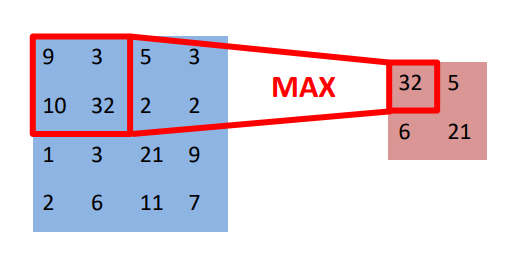
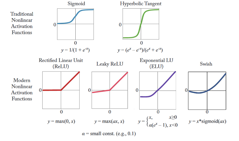
Figure 8 below shows different non-linearity functions. Non-linearity functions, or activation functions, introduce non-linear properties to neural networks, allowing them to learn complex patterns in data. Traditional functions like Sigmoid and Tanh were initially used but suffer from the vanishing gradient problem, which can impede training (they are still used depending on the application). Modern activation functions such as ReLU, Leaky ReLU, ELU, and Swish address this issue by maintaining larger gradients, improving convergence and performance in deep networks. These modern functions are also computationally efficient and help prevent issues like the dying ReLU problem. “Gradient descent” or loss minimization can be visualized in Figure 10, albeit in a different context, one can understand how the center point represents the convergence of low loss and high accuracy of the ML model. In any ML application, and also our medical imaging one, we strive to meet these two objectives.

Traditional Nonlinear Activation Functions

Sigmoid

• Equation: \(y = \frac{1}{1 + e^{-x}}\)
• Description: The sigmoid function outputs values in the range (0, 1). It is commonly used in binary classification problems to model the probability of an output belonging to a certain class. However, it can suffer from the vanishing gradient problem, making it less suitable for deep neural networks.

Hyperbolic Tangent (Tanh)

• Equation: \(y = \frac{e^x - e^{-x}}{e^x + e^{-x}}\)
• Description: The tanh function outputs values in the range (-1, 1). It is zero-centered, which can help with the training of neural networks. Like the sigmoid function, it can also suffer from the vanishing gradient problem, but its output range makes it generally more preferred than sigmoid.

Modern Nonlinear Activation Functions

Rectified Linear Unit (ReLU)

• Equation: \(y = \max(0, x)\)
• Description: The ReLU function outputs the input directly if it is positive; otherwise, it outputs zero. It is one of the most popular activation functions for deep learning because it helps mitigate the vanishing gradient problem and is computationally efficient. However, it can suffer from the “dying ReLU” problem, where neurons can sometimes get stuck during training and always output zero.

Leaky ReLU

• Equation: \(y = \max(ax, x)\) where \(a\) is a small constant (e.g., 0.1)
• Description: Leaky ReLU is a variation of ReLU that allows a small, non-zero gradient when the input is negative. This helps prevent the dying ReLU problem by allowing some gradient to flow through when the input is negative.

Exponential Linear Unit (ELU)

• Equation: \(y = \begin{cases} x & \text{if } x \geq 0 \\ \alpha (e^x - 1) & \text{if } x < 0 \end{cases}\) where \(\alpha\) is a constant.
• Description: ELU is another variation that tends to produce better learning characteristics by smoothing out the curve for negative values, which can lead to faster convergence. The function is zero-centered like tanh but does not suffer from the same vanishing gradient problems as sigmoid and tanh.

Swish

• Equation: \(y = x \cdot \text{sigmoid}(ax)\) where \(a\) is a constant.
• Description: Swish is a newer activation function that has been found to work well in many deep learning applications. It is defined as \(y = x \cdot \text{sigmoid}(x)\) or a scaled version of it. Swish is smooth and non-monotonic, which allows it to perform better on deeper models by maintaining a small gradient for negative inputs.

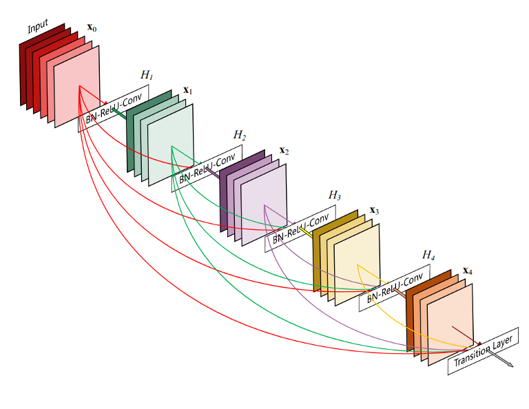
Now that we’ve established the importance of non-linearity functions, we can talk about one of the fundamental features of the U-Net architecture: skip connections (also known as residual connections). They give CNNs the ability to perform better in medical imaging applications. For example, they provide better gradient flow by helping to mitigate the vanishing gradient problem by allowing gradients to flow more easily through the network during backpropagation. As such, the training of these networks can be more effective and is often necessary to be able to capture the complex features in medical imaging. Additionally, there is enhanced feature propagation. By us skipping certain layers, skip connections allow the network to retain and propagate features from earlier layers to later layers to allow the CNN to learn more fine details. Moreover, better convergence is found as more resilient and effective pathways are realized during training. All-in-all, these benefits result in the reduction of overfitting, which is a major concern during the training process of deep neural networks. Loss is reduced and accuracy is uphelp. We will elaborate on the specifics related to skip connections in relation to the SUNS framework soon.

As discussed previously, these optimizations have one goal: reduce loss. Loss represents inadequacies in the learning process. Figure 10 shows this reduction process visually for skip connections (with and without). The loss landscape converges at a global minimum as shown in (b). The minimum is also achieved in (a), but it’s unknown about whether that minimum is correct as the road to the minimum is rough and convergence is often messy. Smooth convergence is desired and results in a higher accuracy, lower loss solution.

CNMF vs. SUNS

Previous tests considered an approach developed by Pnevmatikakis et al. 2016 called Constrained Non-negative Matrix Factorization (CNMF). This was largely used across medical imaging research work to identify and segment neurons.

However, it struggled to accurately segment neurons, often requiring manual correction. Additionally, it required a large amount of image pre-processing prior being sent as an input into the CNMF algorithm. As such, we sought to develop a way to do what CNMF could do, but better and more efficiently. This was the conceptual basis for our work to expand on. The UNet architecture discussed above met these goals with an expansion by Bao et al. 2021 providing a more customized solution for our medical imaging task. For brevity, in-depth discussion of CNMF is not included in this article. More information can be found in the paper by Pnevmatikakis et al. 2016.

The Shallow UNet Neuron Segmentation (SUNS) framework developed by Bao et al. 2021 presents a streamlined version of the U-Net architecture tailored for neuron segmentation in medical imaging. This Shallow UNet retains the core contracting and expanding paths of the traditional U-Net, ensuring accurate segmentation while reducing complexity and computation time. The shallower network design enhances processing speed and efficiency, making it suitable for real-time applications and environments with limited computational resources.

In terms of applicability, SUNS offers a balanced approach by maintaining high segmentation accuracy crucial for identifying intricate neuron structures, while being easier to implement and fine-tune. Its simplified architecture facilitates faster training and inference, benefiting practical deployment in neuron identification tasks. There are however some drawbacks (as with any approach). The main points of CNMF are shown below with respect to algorithm approach, speed and processing, accuracy, feature extraction, and usability/implementation. These points will be shown for SUNS below also to show similarities/differences.

Constrained Non-negative Matrix Factorization

1. Algorithmic Approach: A matrix factorization technique that decomposes fluorescence imaging data into spatial and temporal components. It imposes non-negativity constraints and additional constraints to ensure the physical relevance of the factors. CNMF relies on optimization techniques and linear algebra rather than deep learning.
2. Speed and Real-time Processing: Generally slower as it involves iterative optimization processes. Although it provides accurate results, it is not typically used for real-time applications due to its computational intensity.
3. Accuracy and Handling of Data: Provides accurate segmentation but may struggle with overlapping neurons or low signal-to-noise ratios. It relies on the assumption that the data can be well-represented by a small number of components, which might not always hold true.
4. Feature Extraction: Separates the data into spatial and temporal components but does not inherently integrate advanced pre-processing steps like temporal filtering and whitening. It focuses on decomposing the data matrix into low-rank components.
5. Usability and Implementation: Often requires significant computational resources and expertise in optimization techniques, making it less accessible for real-time applications. It is typically used in post-processing of imaging data.

Shallow UNet Neuron Segmentation

1. Algorithmic Approach: Utilizes a deep learning architecture, specifically a shallow U-Net, designed for image segmentation. It combines temporal filtering and whitening schemes to extract temporal features and uses the U-Net to capture spatial features.
2. Speed and Real-time Processing: Capable of real-time processing, making it significantly faster than traditional methods. It can process videos in real-time, which is crucial for experiments requiring immediate feedback.
3. Accuracy and Handling of Data: Demonstrates higher accuracy, especially in datasets with few manually marked ground truths. The deep learning approach allows it to learn complex features and patterns in the data, leading to better performance in various conditions.
4. Feature Extraction: Extracts both temporal and spatial features through its neural network architecture. Temporal filtering and whitening are used to pre-process the data, enhancing the signal quality before spatial features are extracted by the U-Net.
5. Usability and Implementation: Designed to be user-friendly with the potential for online implementation, allowing researchers to use it directly during experiments. It provides a streamlined workflow for real-time neuron segmentation.

Each of these approaches have their advantages and disadvantages as shown. However, as we will demonstrate, SUNS gives a stronger, more robust framework for future neuron identification work. In addition, CNMF can be used alongside SUNS to pick up where SUNS falls short.

Methods

Baseline and Results

Conclusion